State Estimators

---

source

Bayesian_Filter

def Bayesian_Filter(
    category_sizes:list[int], # Number of states per sensory category.
    sensory_predictions:NDArray[numpy.float64], # Each row is a hypothesis; columns grouped by category_sizes, each group sums to 1.
    transition_predictions:NDArray[numpy.float64], # Each row is a hypothesis; columns give predicted probabilities for each hypothesis being true at the next step.
    belief_prior:NDArray[numpy.float64]=None, # Initial belief prior. If None, set to uniform.
    log_base:float=2.0, # Base for logarithms and exponentials.
    data_record:list[str]=[], # List of internal variable names to record each time step. Accepts "all".
    record_until:int=-1, # Number of time steps to record. Default -1 disables recording.
):

Bayesian Filter for recursive state estimation.

Each state/hypothesis posits: 1. A probability for all states of K sensory categories (with discrete state spaces). 2. A probability that each state/hypothesis will be true when the sensory category states are next updated.

The filter maintains a belief state over these hypotheses/states, assuming they are exhaustive and mutually exclusive.

Bayesian_Filter Example

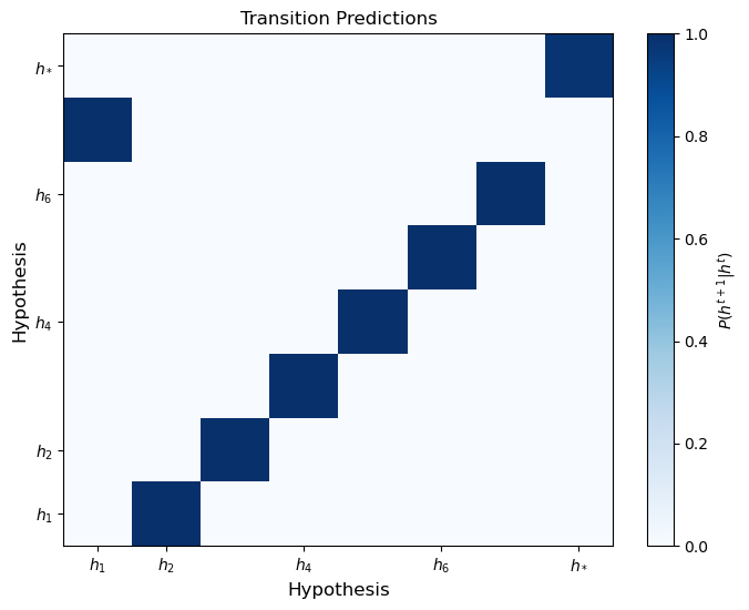
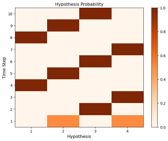
Here we provide a simple example of a Bayesian Filter for an environment in a deterministic cycles. This environment produces the percept sequence “green” “off” “blue” “off”, then repeats.

from projective_simulation.envs.POMDPs import Cyclic_Env
from projective_simulation.methods.visualization import plot_heatmap

np.random.seed(1034300925)
#define percepts
off = 0
green = 1
blue = 2
colormap = np.array(['lightgrey', 'green', 'blue']) #for plotting

#define environment
percept_cycle = np.array([green,off,blue,off]) #light off, light green, light off, light blue
simple_light_cycle = Cyclic_Env(percept_cycle, initial_state = 1) #start with light off to get aliasing


#define agent
category_sizes = [3]
sensory_predictions = simple_light_cycle.observation_function
transition_predictions = simple_light_cycle.transition_function[:,:,0] #Removes action dimension added by environment constructor
test_bayesian_filter = Bayesian_Filter(category_sizes = category_sizes,
                                       sensory_predictions = sensory_predictions,
                                       transition_predictions = transition_predictions
                                      )

#prepare simulation
T = 10 #total time to run simulation
test_bayesian_filter.prepare_data_storage(data_record = ["all"], record_until = T)

#simulate
for t in range(T): #state in light of state to create initial aliasing
    percept = simple_light_cycle.get_observation()
    test_bayesian_filter.sample(percept)
    simple_light_cycle.transition(0) #use action 0

#plot memory trace activations over time
plot_heatmap(test_bayesian_filter.data_dic["belief_posterior"], title = "Hypothesis Probability", color = "Oranges", xlabel = "Hypothesis") # type: ignore

Memory-Based State Estimators

---

source

Sequence_Memory

def Sequence_Memory(
    category_sizes:list[int], # Number of states for each sensor/percept category.
    memory_capacity:int, # Number of memory-based hypotheses.
    memory_bias:float, # Probability of transitioning from non-memory to memory hypothesis space.
    stationary_expectations:NDArray[numpy.float64]=None, # Expectation of sensory states in stationarity. Default to uniform distributions for each sensor.
    sensory_predictions:NDArray[numpy.float64]=None, # Sensory hypotheses matrix. If None, initialized to uniform.
    belief_prior:NDArray[numpy.float64]=None, # Initial belief priors. If None, all prior on non-memory hypothesis.
    transition_predictions:NDArray[numpy.float64]=None, # Hypothesis transition matrix.
    next_trace:int=0, # Starting memory index. 0 means no memory traces encoded yet.
    capacity_overflow_method:str='stop encoding', # 'loop' or 'stop encoding'.
    data_record:list[str]=[], # List of variable names to log each time step. Accepts "all".
    record_until:int=-1, # Number of steps to prepare for data logging. Negative disables recording.
    stationary_transition_method:str='first', # 'encoded', 'first', or 'learned'.
):

Memory-based Bayesian filter that encodes a sequence of percepts as memory traces. Each memory trace is a hypothesis about the environment, and the agent can transition between non-memory and memory hypotheses. Memory traces are encoded by dynamic modification of transition function and observation function.

Sequence_Memory Example

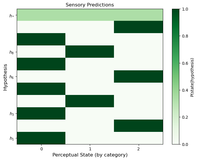
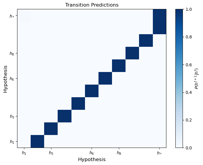
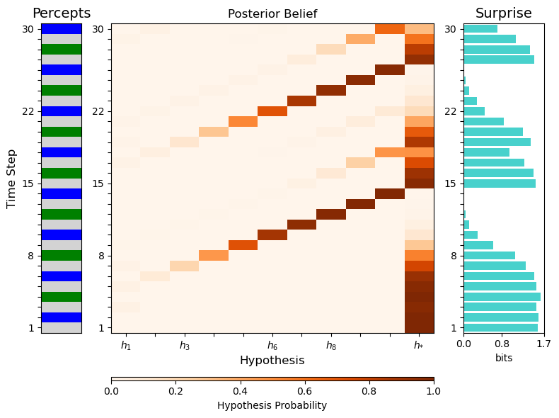
In this example, set up a cyclical Hidden Markov Process in which a light turns green, turns off, turns blue, turns off, then turns green again and restarts. We show how to pass the percepts from this environment to the Memory Network, record the network’s internal states over time, and visualize these states after simuluation.

from projective_simulation.envs.POMDPs import Cyclic_Env
from projective_simulation.methods.visualization import plot_heatmap, memory_filter_performance

np.random.seed(1033300925)

#define percepts
off = 0
green = 1
blue = 2
colormap = np.array(['lightgrey', 'green', 'blue']) #for plotting

#define environment
percept_cycle = np.array([green,off,blue,off]) #light off, light green, light off, light blue
simple_light_cycle = Cyclic_Env(percept_cycle, initial_state = 1) #start with light off to get aliasing


#define agent
category_sizes = [3]
memory_capacity = 10
memory_bias = 0.01
test_sequence_memory = Sequence_Memory(
    category_sizes = category_sizes,
    memory_capacity = memory_capacity,
    memory_bias = memory_bias
)

#prepare simulation
T = 30 #total time to run simulation
test_sequence_memory.prepare_data_storage(data_record = ["all"], record_until = T)

#simulate
percepts = [None] * T
for t in range(T):
    percepts[t] = simple_light_cycle.get_observation()
    test_sequence_memory.sample(percepts[t])
    simple_light_cycle.transition(0) #Use action 0 for no-action environments

#plot memory trace activations over time
memory_filter_performance(test_sequence_memory.data_dic, percepts, colormap)

No stationary_expectations given, using uniform distributions for all sensors

test_sequence_memory.show_sensory_predictions()

test_sequence_memory.show_transition_predictions()

---

source

Short_Term_Memory

def Short_Term_Memory(
    category_sizes:list[int], # Number of states each sensor/percept category can take
    memory_capacity:int, # Number of memory nodes.
    memory_bias:float, # Transition probability from non-memory to memory hypothesis.
    fading_rate:float, # Rate parameter for exponential decay toward uniform for memory traces.
    stationary_expectations:NDArray[numpy.float64]=None, # Expectation of sensory states in stationarity. Default to uniform distributions for each sensor.
    sensory_predictions:NDArray[numpy.float64]=None, # Optional sensory-to-memory weight matrix.
    belief_prior:NDArray[numpy.float64]=None, # Optional 1d array of prior expectations on memories.
    transition_predictions:NDArray[numpy.float64]=None, # Optional memory transition matrix.
    next_trace:int=0, # Starting memory index. 0 indicates no memories encoded.
    data_record:list[str]=[], # List of variable names to record each time step. Accepts "all".
    record_until:int=-1, # Number of steps to prepare for data recording. Negative disables recording.
    capacity_overflow_method:str='loop', # 'loop' or 'stop encoding'.
    stationary_transition_method:str='encoded', # 'encoded', 'first', or 'learned'.
):

Short-Term Memory extends Sequence_Memory by introducing memory fading. Each encoded memory trace fades toward the stationary sensory predictions at a specified rate. Supports different schematic transition methods and capacity overflow behaviors.

Short_Term_Memory Example

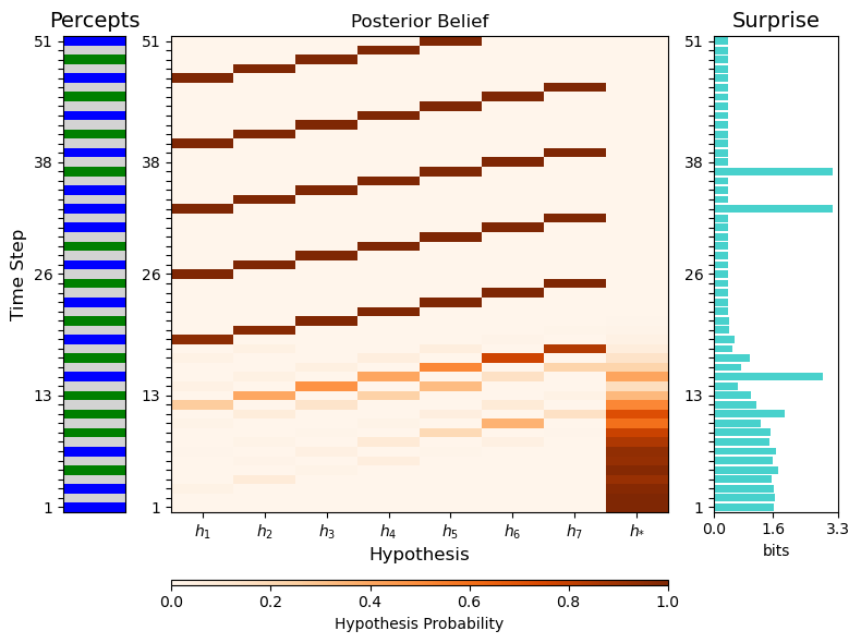
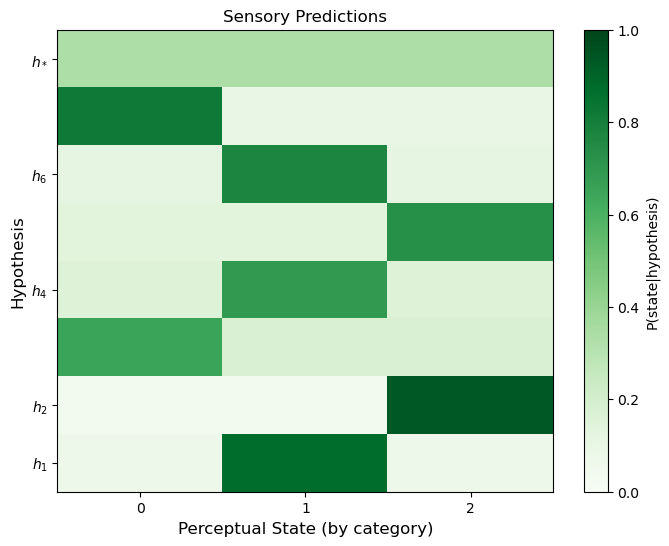
Short-Term memory filters can perfrom state estimations in cyclic environments with certain amounts of noise. Here, we simulate short-term memory in an environment that produces a green-off-blue-off cycle, but where the green/blue color signal is subject to error. We then evaluate the belief state dynamics of this network with a function that plots the time evolution of percept, posterior belief state, and suprise side-by-side. Finally, to illustrate how the observation function changes in short-term memory, we visualize the observation function at the end of the cycle. When compared to the sequence memory, this example illustrates how short-term memory can handle certain kinds of noise in an environment.

from projective_simulation.envs.POMDPs import Noisy_Cycle
from projective_simulation.methods.visualization import plot_heatmap
from projective_simulation.methods.visualization import memory_filter_performance

np.random.seed(1032300925)
#define percepts
green = 0
off = 1
blue = 2
colormap = np.array(['green','lightgrey', 'blue']) #for plotting

#define environment
percepts = np.array([0,1,2])
observation_function = np.array([[0.9,0.,0.1],
                                 [0.,1.,0.],
                                 [0.1,0.,0.9],
                                 [0.,1.,0.]])
noisy_light_cycle = Noisy_Cycle(percepts, observation_function)

#define agent
category_sizes = [3]
memory_capacity = 7
memory_bias = 0.02
fading_rate = 0.1 #this is fast, for the sake of example
test_stm = Short_Term_Memory(
    category_sizes=category_sizes,
    memory_capacity=memory_capacity,
    memory_bias=memory_bias,
    fading_rate=fading_rate,
    stationary_transition_method="encoded",
    capacity_overflow_method="decay_based"
)


#prepare simulation
T = 51 #total time to run simulation
observed_percepts = [None] * T #data structure for storing observations
test_stm.prepare_data_storage(data_record = ["all"], record_until = T)

#simulate for T steps and store observations
for t in range(T):
    percept = noisy_light_cycle.get_observation()
    observed_percepts[t] = percept
    test_stm.sample(percept)  
    noisy_light_cycle.transition(0) #use action 0 for env with no action control

No stationary_expectations given, using uniform distributions for all sensors

memory_filter_performance(memory_data=test_stm.data_dic, 
                          observed_percepts=observed_percepts, 
                          colormap=colormap)

test_stm.show_sensory_predictions()

test_stm.show_transition_predictions()

---

source

Long_Term_Memory

def Long_Term_Memory(
    category_sizes:list[int], # Number of states each sensor/percept category can take
    memory_capacity:int, # Number of memory nodes.
    memory_bias:float, # Transition probability from non-memory to memory hypothesis.
    fading_rate:float, # Base rate parameter for exponential decay toward uniform for memory traces.
    surprise_factor:float=0.0, # Scales the degree to which surprise slows down memory fading.
    consolidation_rate:float=0.0, # Scales the degree to which reactivation slows fading.
    stationary_expectations:NDArray[numpy.float64]=None, # Expectation of sensory states in stationarity. Default to uniform distributions for each sensor.
    sensory_predictions:NDArray[numpy.float64]=None, # Optional sensory-to-memory weight matrix.
    belief_prior:NDArray[numpy.float64]=None, # Optional 1d array of prior expectations on memories.
    transition_predictions:NDArray[numpy.float64]=None, # Optional memory transition matrix.
    next_trace:int=0, # Starting memory time index. 0 indicates no memories encoded.
    data_record:list[str]=[], # List of variable names to record each time step. Accepts "all".
    record_until:int=-1, # Number of steps to prepare for data recording. Negative disables recording.
    fading_rate_method:str='sigmoid', # Method for computing fading rates ("sigmoid" or "surprise_advantage").
    capacity_overflow_method:str='stop encoding', # 'loop' or 'stop encoding'.
    stationary_transition_method:str='encoded', # 'encoded', 'first', or 'learned'.
):

Long_Term_Memory extends Short_Term_Memory by introducing surprise-modulated memory fading and memory stabilization. Each encoded memory trace fades toward a given (estimated) stationary distribution at a rate modulated by the surprise of the encoded percept and by reactivation. Reactivation slows fading and can reinforce the memory trace, stabilizing early memories of sequences.

Long_Term_Memory Example

When the environment does not tend to repeat percepts in a cycle of fixed length, or sequences are long, short-term memory often fails. Here, we define changes to the memory that introduce Long-Term Memory. The long term memory filter encodes the surprise of each sensory state into a memory trace - higher surprise slows fading and thus increases the probability of reactivation upon a similar state. Reactivation also causes the sensory predictions of the memory to mix with current sensory activations - typically reinforcing the memory and counter-acting fading. Together, these dynamics stablize early memories of sequences.

Here, we build an environment that alternates between three sequences of different lengths. Each sequence befins with either ‘green’, ‘blue’, or ‘red’. The color indicates how many time steps of ‘off’ will occur before the ‘black’ percept. A new sequence then begins at random. We visualize the final observation function of Long-Term Memory simulated in such an environment show how the Long-Term Memory retains surprising memories. Note, for example, the fading of memories after time-step forty, when a sequence similar to the first one observed by the Long-Term Memory repeats.

from projective_simulation.envs.POMDPs import POMDP
from projective_simulation.methods.visualization import memory_filter_performance
from projective_simulation.methods.visualization import plot_heatmap

np.random.seed(1029300925)
#define percepts
off = 0
green = 1
blue = 2
red = 3
black = 4
colormap = np.array(['lightgrey', 'green', 'blue', 'red', 'black']) #for plotting

#define environment
percepts = np.array([0,1,2,3,4])
#set up environment
observation_function = np.array([(0.,1.,0.,0.,0.),
                                 (0.,0.,0.,0.,1.),
                                 (0.,0.,1.,0.,0.),
                                 (1.,0.,0.,0.,0.),
                                 (0.,0.,0.,0.,1.),
                                 (0.,0.,0.,1.,0.),
                                 (1.,0.,0.,0.,0.),
                                 (1.,0.,0.,0.,0.),
                                 (0.,0.,0.,0.,1.),
                                ])
transition_function = np.array([(0.,1.,0.,0.,0.,0.,0.,0.,0.),
                                (1/3,0.,1/3,0.,0.,1/3,0.,0.,0.),
                                (0.,0.,0.,1.,0.,0.,0.,0.,0.),
                                (0.,0.,0.,0.,1.,0.,0.,0.,0.),
                                (1/3,0.,1/3,0.,0.,1/3,0.,0.,0.),
                                (0.,0.,0.,0.,0.,0.,1.,0.,0.),
                                (0.,0.,0.,0.,0.,0.,0.,1.,0.),
                                (0.,0.,0.,0.,0.,0.,0.,0.,1.),
                                (1/3,0.,1/3,0.,0.,1/3,0.,0.,0.)
                               ])

alternating_cycles = POMDP(percepts = percepts, 
                           observation_function = observation_function, 
                           transition_function = transition_function[:,:,np.newaxis])

#set up memory filter
category_sizes = [5]
memory_capacity = 80
memory_bias = 0.001
fading_rate = 0.01
consolidation_rate = 0.1
surprise_factor = 0.95

#give schematic hypothesis and unencoded memories default sensory predictions equal to stationary expectation
sensory_predictions = np.tile([3/9,1/9,1/9,1/9, 3/9], (memory_capacity + 1, 1))

test_ltm = Long_Term_Memory(category_sizes = category_sizes,
                            memory_capacity = memory_capacity,
                            memory_bias = memory_bias,
                            sensory_predictions = sensory_predictions,
                            fading_rate = fading_rate,
                            consolidation_rate = consolidation_rate, 
                            surprise_factor = surprise_factor,
                            capacity_overflow_method="decay_based"
                           )

#prepare simulation
T = 80 #total time to run simulation
observed_percepts = [None] * T #data structure for storing observations
test_ltm.prepare_data_storage(data_record = ["all"], record_until = T)

#simulate
for t in range(T):
    percept = alternating_cycles.get_observation()
    observed_percepts[t] = percept
    test_ltm.sample(percept)
    alternating_cycles.transition(0) #use action 0 for environments with no action mediation

memory_filter_performance(memory_data=test_ltm.data_dic, 
                          observed_percepts=observed_percepts, 
                          colormap=colormap)

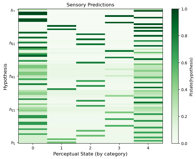
#Plot sensory predictions. Note that the oldest memories tend to be "sharper" then middle-age memories.
test_ltm.show_sensory_predictions()

test_ltm.show_transition_predictions()

---

source

Associative_Memory

def Associative_Memory(
    category_sizes:list[int], # Number of states each sensor/percept category can take
    memory_capacity:int, # Number of memory nodes.
    memory_bias:float, # Transition probability from non-memory to memory hypothesis.
    fading_rate:float, # Base rate parameter for exponential decay toward uniform for memory traces.
    surprise_factor:float=0.0, # Scales the degree to which surprise slows down memory fading.
    consolidation_rate:float=0.0, # Scales the degree to which reactivation slows fading.
    reassociation_rate:float=0.0, # Scales influence of prediction differences on transition weights.
    reencoding_rate:float=0.0, # Scales the degree to which re-activation of a memory affects its sensory predictions.
    stationary_expectations:NDArray[numpy.float64]=None, # Expectation of sensory states in stationarity. Default to uniform distributions for each sensor.
    sensory_predictions:NDArray[numpy.float64]=None, # Optional sensory-to-memory weight matrix.
    belief_prior:NDArray[numpy.float64]=None, # Optional 1d array of prior expectations on memories.
    transition_predictions:NDArray[numpy.float64]=None, # Optional memory transition matrix.
    next_trace:int=0, # Starting memory time index. 0 indicated no memories encoded
    data_record:list[str]=[], # List of variable names to record each time step. Accepts "all".
    record_until:int=-1, # Number of steps to prepare for data recording. Negative disables recording.
    fading_rate_method:str='sigmoid', # Method for computing fading rates ("sigmoid" or "surprise_advantage").
    capacity_overflow_method:str='decay_based', # 'loop', 'stop encoding', or decay_based.
    stationary_transition_method:str='learned', # 'encoded', 'first', or 'learned'.
):

Associative_Memory extends Long_Term_Memory by introducing learning and re-encoding mechanisms. This class allows memory traces to be updated based on prediction differences (reassociation_rate) and reactivation (reencoding_rate). Transition weights between memory traces can be learned, and reactivation can reinforce or generalize memory traces.

Associative_Memory Example

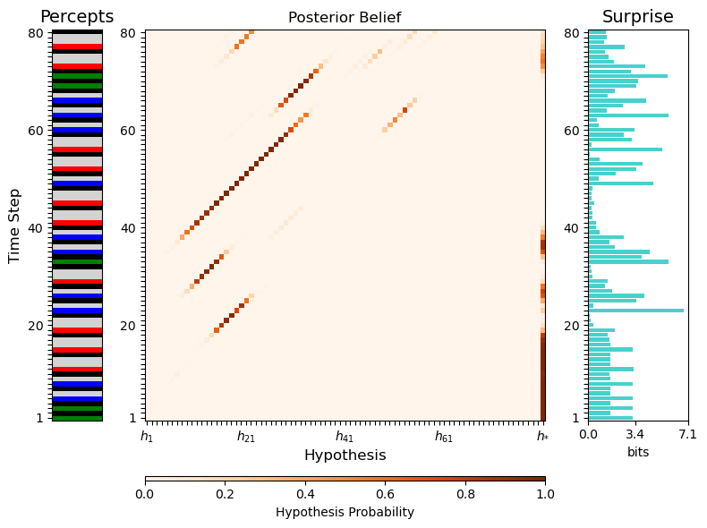
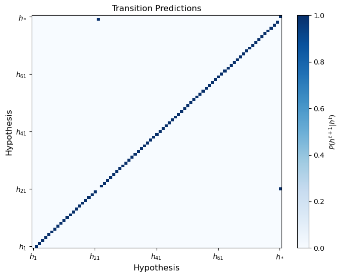
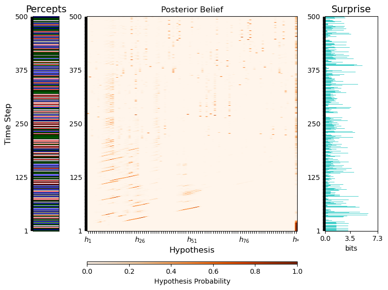
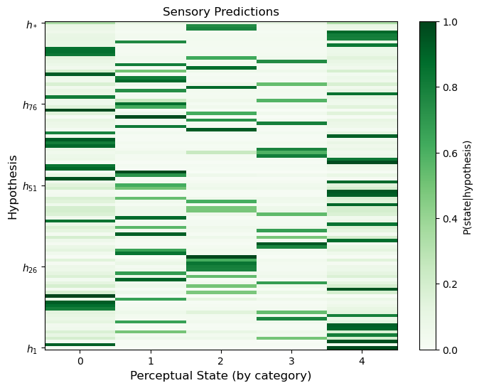
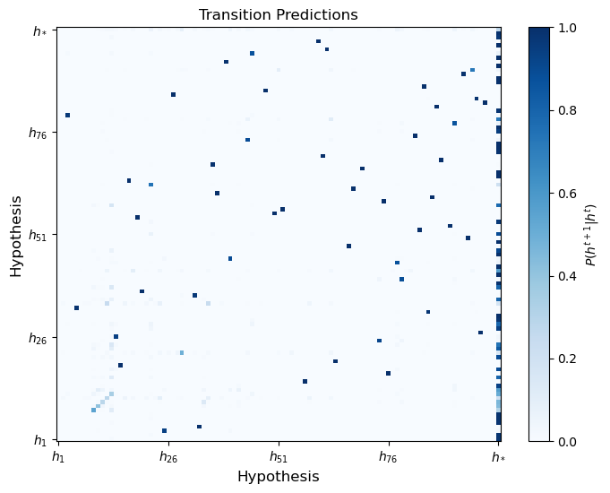
Here, we simulate Associative Memory in an environment that alternates between three sequences of different lengths. Each sequence befins with either ‘green’, ‘blue’, or ‘red’. The color indicates how many time steps of ‘off’ will occur before the ‘black’ percept. A new sequence then begins at random. We visualize the time evolution of the belief state of Associative memory side-by-side with the percept sequence and according surprise of the Associative Memory. Then we visualize the final observation function and a portion of the final transition function of the Associative Memory. When compared to the Long-Term Memory, this example illustrates how associative memory uses the plasticity of memory traces to learn about stochastic transitions in the environment, leading memory traces of later experiences where it already understands the environment to fade.

from projective_simulation.envs.POMDPs import POMDP
from projective_simulation.methods.visualization import memory_filter_performance
from projective_simulation.methods.visualization import plot_heatmap

np.random.seed(1035300925)
#define percepts
off = 0
green = 1
blue = 2
red = 3
black = 4

#define environment
percepts = np.array([0,1,2,3,4])
#set up environment
observation_function = np.array([(0.,1.,0.,0.,0.),
                                 (0.,0.,0.,0.,1.),
                                 (0.,0.,1.,0.,0.),
                                 (1.,0.,0.,0.,0.),
                                 (0.,0.,0.,0.,1.),
                                 (0.,0.,0.,1.,0.),
                                 (1.,0.,0.,0.,0.),
                                 (1.,0.,0.,0.,0.),
                                 (0.,0.,0.,0.,1.),
                                ])
transition_function = np.array([(0.,1.,0.,0.,0.,0.,0.,0.,0.),
                                (1/3,0.,1/3,0.,0.,1/3,0.,0.,0.),
                                (0.,0.,0.,1.,0.,0.,0.,0.,0.),
                                (0.,0.,0.,0.,1.,0.,0.,0.,0.),
                                (1/3,0.,1/3,0.,0.,1/3,0.,0.,0.),
                                (0.,0.,0.,0.,0.,0.,1.,0.,0.),
                                (0.,0.,0.,0.,0.,0.,0.,1.,0.),
                                (0.,0.,0.,0.,0.,0.,0.,0.,1.),
                                (1/3,0.,1/3,0.,0.,1/3,0.,0.,0.)
                               ])

alternating_cycles = POMDP(percepts = percepts, 
                           observation_function = observation_function, 
                           transition_function = transition_function[:,:,np.newaxis])

#set up memory filter
category_sizes = [5]
memory_capacity = 100
memory_bias = 0.0001
fading_rate = 0.004
consolidation_rate = 0.2
surprise_factor = 0.99
reencoding_rate = 0.2
reassociation_rate = 0.2

#give schematic hypothesis and unencoded memories default sensory predictions equal to stationary expectation
sensory_predictions = np.tile([3/9,1/9,1/9,1/9, 3/9], (memory_capacity + 1, 1))

test_am = Associative_Memory(category_sizes = category_sizes,
                          memory_capacity = memory_capacity,
                          memory_bias = memory_bias,
                          sensory_predictions = sensory_predictions,
                          fading_rate = fading_rate,
                          consolidation_rate = consolidation_rate,
                          reencoding_rate = reencoding_rate,
                          surprise_factor = surprise_factor,
                          reassociation_rate = reassociation_rate,
                          capacity_overflow_method="decay_based"
                         )

#prepare simulation
T = 500 #total time to run simulation
observed_percepts = ["None"] * T #data structure for storing observations
test_am.prepare_data_storage(data_record = ["all"], record_until = T)

#simulate
for t in range(T):
    percept = alternating_cycles.get_observation()
    observed_percepts[t] = percept
    test_am.sample(percept)
    alternating_cycles.transition(0) #use action 0 for environments with no action mediation

memory_filter_performance(memory_data=test_am.data_dic, 
                          observed_percepts=observed_percepts, 
                          colormap=colormap)

#Plot sensory predictions. Note that the oldest memories tend to be "sharper" then middle-age memories.
test_am.show_sensory_predictions()

#Plot transition predictions
test_am.show_transition_predictions()

test_am.transition_predictions[-1,:]

array([1.34644910e-04, 7.13974030e-03, 8.09562209e-03, 6.94895460e-03,
       4.44671688e-03, 1.85399371e-04, 8.47119985e-03, 7.73742164e-03,
       1.09235153e-02, 0.00000000e+00, 1.05925418e-02, 1.15354485e-04,
       6.09689595e-03, 2.15525986e-03, 9.60581741e-03, 8.14354884e-03,
       1.45064863e-04, 7.23422754e-03, 6.93685545e-03, 1.03092260e-03,
       9.41828295e-03, 1.11125173e-04, 4.51894581e-04, 1.28210332e-02,
       4.31843998e-03, 7.23827773e-03, 2.44386048e-04, 6.79138438e-03,
       3.42624021e-03, 2.60443527e-03, 2.46882835e-02, 6.72578925e-04,
       1.15946518e-02, 9.90099010e-03, 3.22357398e-02, 1.55588378e-03,
       7.95449369e-03, 5.64208025e-03, 3.34567018e-04, 1.35692962e-02,
       1.61006327e-02, 1.01474435e-02, 2.15076603e-02, 6.71728538e-03,
       6.69258639e-04, 9.12744390e-03, 9.04208396e-03, 6.82846410e-03,
       1.10195445e-02, 8.44776830e-03, 8.77949546e-04, 4.16145988e-03,
       8.63024445e-04, 3.23005048e-04, 2.76091282e-05, 4.41396287e-03,
       5.69217196e-03, 1.02237007e-03, 3.99364579e-03, 6.55771984e-03,
       1.08091086e-03, 1.85417081e-03, 7.26011712e-04, 1.82813681e-03,
       1.86526494e-03, 6.87380277e-03, 3.91124345e-05, 5.50735959e-02,
       7.22691160e-03, 2.49528748e-04, 8.48475222e-05, 7.68084625e-03,
       3.20103252e-03, 6.65219839e-03, 5.11773965e-03, 6.65827107e-03,
       9.29176331e-03, 1.44797717e-03, 5.27277271e-05, 2.57350934e-04,
       1.69332380e-03, 1.52160157e-02, 3.85795850e-02, 9.74211697e-03,
       6.48013801e-03, 4.22471016e-03, 1.90876215e-03, 6.72073168e-03,
       1.29812033e-02, 8.20690774e-03, 1.63325112e-03, 3.79448559e-04,
       1.54877746e-02, 3.42765486e-03, 9.36414899e-03, 8.97663795e-03,
       1.10127084e-02, 1.18576342e-02, 2.28224597e-04, 7.57749787e-04,
       3.24604799e-01])

nbdev export